24. Neural Network Regression with JAX#
GPU
This lecture was built using a machine with access to a GPU — although it will also run without one.
Google Colab has a free tier with GPUs that you can access as follows:
Click on the “play” icon top right
Select Colab
Set the runtime environment to include a GPU
24.1. Outline#
In a previous lecture, we showed how to implement regression using a neural network via the deep learning library Keras.
In this lecture, we solve the same problem directly, using JAX operations rather than relying on the Keras frontend.
The objectives are
Understand the nuts and bolts of the exercise better
Explore more features of JAX
Observe how using JAX directly allows us to greatly improve performance.
The lecture proceeds in three stages:
We solve the problem using Keras, to give ourselves a benchmark.
We solve the same problem in pure JAX, using pytree operations and gradient descent.
We solve the same problem using a combination of JAX and Optax, an optimization library built for JAX.
We begin with imports and installs.
import jax
import jax.numpy as jnp
import matplotlib.pyplot as plt
import os
from time import time
from typing import NamedTuple
from functools import partial
!pip install keras optax
os.environ['KERAS_BACKEND'] = 'jax'
import keras
from keras import Sequential
from keras.layers import Dense
import optax
24.2. Set up#
Here we briefly describe the problem and generate synthetic data.
24.2.1. Flow#
We use the routine from Simple Neural Network Regression with Keras and JAX to generate data for one-dimensional nonlinear regression.
Then we will create a dense (i.e., fully connected) neural network with 4 layers, where the input and hidden layers map to \(k\)-dimensional output space.
The inputs and outputs are scalar (for one-dimensional nonlinear regression), so the overall mapping is
Here’s a class to store the learning-related constants we’ll use across all implementations.
Our default value of \(k\) will be 10.
class Config(NamedTuple):
    epochs: int = 4000             # Number of passes through the data set
    learning_rate: float = 0.001   # Learning rate for gradient descent
    layer_sizes: tuple = (1, 10, 10, 10, 1)  # Layer sizes
    seed: int = 14                 # Random seed for data generation
24.2.2. Data#
Here’s the function to generate the data for our regression analysis.
def generate_data(
        key: jax.Array,         # JAX random key
        data_size: int = 400,   # Sample size
        x_min: float = 0.0,     # Minimum x value
        x_max: float = 5.0      # Maximum x value
    ):
    """
    Generate synthetic regression data.
    """
    x = jnp.linspace(x_min, x_max, num=data_size)
    ϵ = 0.2 * jax.random.normal(key, shape=(data_size,))
    y = x**0.5 + jnp.sin(x) + ϵ
    # Return observations as column vectors
    x = jnp.reshape(x, (data_size, 1))
    y = jnp.reshape(y, (data_size, 1))
    return x, y
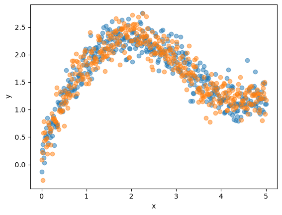
Here’s a plot of the data.
config = Config()
key = jax.random.key(config.seed)
key_train, key_validate = jax.random.split(key)
x_train, y_train = generate_data(key_train)
x_validate, y_validate = generate_data(key_validate)
keras.utils.set_random_seed(config.seed)
fig, ax = plt.subplots()
ax.scatter(x_train, y_train, alpha=0.5)
ax.scatter(x_validate, y_validate, alpha=0.5)
ax.set_xlabel('x')
ax.set_ylabel('y')
plt.show()
24.3. Training with Keras#
We build a Keras model that can fit a nonlinear function to the generated data using an ANN.
We will use this fit as a benchmark to test our JAX code.
Since its role is only a benchmark, we refer readers to the previous lecture for details on the Keras interface.
We start with a function to build the model.
def build_keras_model(
        config: Config,                     # contains configuration data
        activation_function: str = 'tanh'   # activation with default
    ):
    model = Sequential()
    layer_sizes = config.layer_sizes

    # Add layers to the network sequentially, from inputs towards outputs
    for in_dim, out_dim in zip(layer_sizes[:-2], layer_sizes[1:-1]):
        model.add(
           Dense(
               units=out_dim,
               activation=activation_function,
               kernel_initializer=keras.initializers.HeNormal(),
               bias_initializer='ones',
           )
        )
    # Add a final layer that maps to a scalar value, for regression.
    model.add(
        Dense(
            units=layer_sizes[-1],
            kernel_initializer=keras.initializers.HeNormal(),
            bias_initializer='ones',
        )
    )
    # Embed training configurations
    model.compile(
        optimizer=keras.optimizers.SGD(
            learning_rate=config.learning_rate
        ),
        loss='mean_squared_error'
    )
    return model
Notice that we’ve set the optimizer to use stochastic gradient descent and a mean square loss.
Here is a function to train the model.
def train_keras_model(
        model,          # Instance of Keras Sequential model
        x,              # Training data, inputs
        y,              # Training data, outputs
        x_validate,     # Validation data, inputs
        y_validate,     # Validation data, outputs
        config: Config  # contains configuration data
    ):
    print("Training NN using Keras.")
    start_time = time()
    training_history = model.fit(
        x, y,
        batch_size=max(x.shape),
        verbose=0,
        epochs=config.epochs,
        validation_data=(x_validate, y_validate)
    )
    elapsed = time() - start_time
    mse = model.evaluate(x_validate, y_validate, verbose=2)
    print(f"Trained in {elapsed:.2f} seconds, validation data MSE = {mse}")
    return model, training_history, elapsed, mse
The next function extracts and visualizes a prediction from the trained Keras model.
def plot_keras_output(model, x_validate, y_validate):
    y_predict = model.predict(x_validate, verbose=2)
    fig, ax = plt.subplots()
    ax.scatter(x_validate, y_validate, alpha=0.5)
    ax.plot(x_validate, y_predict, label="fitted model", color='black')
    ax.set_xlabel('x')
    ax.set_ylabel('y')
    plt.show()
Let’s run the Keras training:
config = Config()
model = build_keras_model(config)
model, training_history, keras_runtime, keras_mse = train_keras_model(
    model, x_train, y_train, x_validate, y_validate, config
)
plot_keras_output(model, x_validate, y_validate)
Training NN using Keras.
13/13 - 0s - 29ms/step - loss: 0.0464
Trained in 21.58 seconds, validation data MSE = 0.0464036725461483
13/13 - 0s - 23ms/step
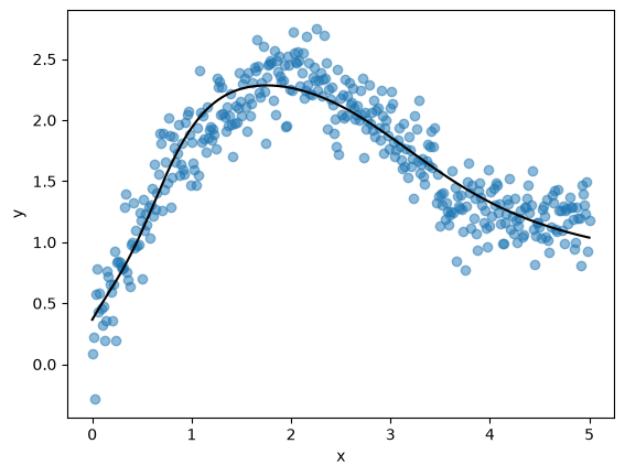
The fit is good and we note the relatively low final MSE.
24.4. Training with JAX#
For the JAX implementation, we need to construct the network ourselves, as a map from inputs to outputs.
We’ll use the same network structure we used for the Keras implementation.
24.4.1. Background and set up#
The neural network has the form
Here
\( x \) is a scalar input – a point on the horizontal axis in the Keras estimation above,
\( \circ \) means composition of maps,
\( \sigma \) is the activation function – in our case, \( \tanh \), and
\( A_i \) represents the affine map \( A_i x = W_i x + b_i \).
Each matrix \( W_i \) is called a weight matrix and each vector \( b_i \) is called a bias term.
The symbol \( \theta \) represents the entire collection of parameters:
In fact, when we implement the affine map \( A_i x = W_i x + b_i \), we will work with row vectors rather than column vectors, so that
\( x \) and \( b_i \) are stored as row vectors, and
the mapping is executed by JAX via the expression
x @ W + b.
Here’s a class to store parameters for one layer of the network.
class LayerParams(NamedTuple):
    """
    Stores parameters for one layer of the neural network.

    """
    W: jax.Array     # weights
    b: jax.Array     # biases
The following function initializes a single layer of the network using He initialization for weights and ones for biases.
def initialize_layer(in_dim, out_dim, key):
    """
    Initialize weights and biases for a single layer of the network.
    Use He initialization for weights and ones for biases.
    """
    W = jax.random.normal(key, shape=(in_dim, out_dim)) * jnp.sqrt(2 / in_dim)
    b = jnp.ones((1, out_dim))
    return LayerParams(W, b)
The next function builds an entire network, as represented by its parameters, by initializing layers and stacking them into a list.
def initialize_network(
        key: jax.Array,     # JAX random key
        config: Config      # contains configuration data
    ):
    """
    Build a network by initializing all of the parameters.
    A network is a list of LayerParams instances, each
    containing a weight-bias pair (W, b).
    """
    layer_sizes = config.layer_sizes
    params = []
    for i in range(len(layer_sizes) - 1):
        key, subkey = jax.random.split(key)
        layer = initialize_layer(
            layer_sizes[i],      # in dimension for layer
            layer_sizes[i + 1],  # out dimension for layer
            subkey
        )
        params.append(layer)
    return params
Wait, you say!
Shouldn’t we concatenate the elements of \(\theta\) into some kind of big array, so that we can do autodiff with respect to this array?
Actually we don’t need to — we use the JAX PyTree approach discussed below.
24.4.2. Coding the network#
Here’s our implementation of the ANN \(f\):
def f(
        θ: list,                        # Network parameters (pytree)
        x: jax.Array,                 # Input data (row vector)
        σ: callable = jnp.tanh          # Activation function
    ):
    """
    Perform a forward pass over the network to evaluate f(θ, x).
    """
    *hidden, last = θ
    for layer in hidden:
        x = σ(x @ layer.W + layer.b)
    x = x @ last.W + last.b
    return x
The function \(f\) is appropriately vectorized, so that we can pass in the entire
set of input observations as x and return the predicted vector of outputs y_hat = f(θ, x)
corresponding to each data point.
The loss function is mean squared error, the same as the Keras case.
def loss_fn(
        θ: list,            # Network parameters (pytree)
        x: jax.Array,     # Input data
        y: jax.Array      # Target data
    ):
    return jnp.mean((f(θ, x) - y)**2)
We’ll also define a function to visualize predictions from our JAX models.
def plot_jax_output(θ, x_validate, y_validate):
    fig, ax = plt.subplots()
    ax.scatter(x_validate, y_validate, color='red', alpha=0.5)
    ax.plot(x_validate.flatten(), f(θ, x_validate).flatten(),
            label="fitted model", color='black')
    ax.set_xlabel('x')
    ax.set_ylabel('y')
    plt.show()
We’ll use the gradient of the loss to do stochastic gradient descent.
(Technically, we will be doing gradient descent, rather than stochastic gradient descent, since we will not randomize over sample points when we evaluate the gradient.)
loss_gradient = jax.grad(loss_fn)
The gradient of loss_fn is with respect to the first argument θ.
The code above seems kind of magical, since we are differentiating with respect to a parameter “vector” stored as a list of namedtuples containing arrays.
How can we differentiate with respect to such a complex object?
The answer is that the list of namedtuples is treated internally as a pytree.
The JAX function grad understands how to
extract the individual arrays (the “leaves” of the tree),
compute derivatives with respect to each one, and
pack the resulting derivatives into a pytree with the same structure as the parameter vector.
24.4.3. Gradient descent#
Using the above code, we can now write our rule for updating the parameters via gradient descent, which is the algorithm we covered in our lecture on autodiff.
In this case, to keep things as simple as possible, we’ll use a fixed learning rate for every iteration.
def update_parameters(
        θ: list,            # Current parameters (pytree)
        x: jax.Array,     # Input data
        y: jax.Array,     # Target data
        config: Config      # contains configuration data
    ):
    """
    Update the parameter pytree using gradient descent.

    """
    λ = config.learning_rate

    # Specify the update rule
    def gradient_descent_step(p, g):
        """
        A rule for updating parameter vector p given gradient vector g.
        It will be applied to each leaf of the pytree of parameters.
        """
        return p - λ * g

    gradient = loss_gradient(θ, x, y)

    # Use tree.map to apply the update rule to the parameter vectors
    θ_new = jax.tree.map(gradient_descent_step, θ, gradient)
    return θ_new
Here jax.tree.map understands θ and gradient as pytrees of the
same structure and executes p - λ * g on the corresponding leaves of the pair
of trees.
Each weight matrix and bias vector is updated by gradient descent, exactly as required.
Here’s code that puts this all together.
@partial(jax.jit, static_argnames=['config'])
def train_jax_model(
        θ: list,                    # Initial parameters (pytree)
        x: jax.Array,             # Training input data
        y: jax.Array,             # Training target data
        config: Config              # contains configuration data
    ):
    """
    Train model using gradient descent.
    """
    def update(_, θ):
        θ_new = update_parameters(θ, x, y, config)
        return θ_new

    θ_final = jax.lax.fori_loop(0, config.epochs, update, θ)
    return θ_final
24.4.4. Execution#
Let’s run our code and see how it goes.
We’ll reuse the data we generated earlier.
# Reset parameter vector
config = Config()
param_key = jax.random.key(1234)
θ = initialize_network(param_key, config)

# Warmup run to trigger JIT compilation
train_jax_model(θ, x_train, y_train, config)

# Reset and time the actual run
θ = initialize_network(param_key, config)
start_time = time()
θ = train_jax_model(θ, x_train, y_train, config)
θ[0].W.block_until_ready()  # Ensure computation completes
jax_runtime = time() - start_time

jax_mse = loss_fn(θ, x_validate, y_validate)
jax_train_mse = loss_fn(θ, x_train, y_train)
print(f"Trained model with JAX in {jax_runtime:.2f} seconds.")
print(f"Final MSE on validation data = {jax_mse:.6f}")
Trained model with JAX in 0.25 seconds.
Final MSE on validation data = 0.042119
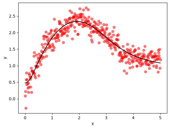
Despite the simplicity of our implementation, we actually perform slightly better than Keras.
Here’s a visualization of the quality of our fit.
plot_jax_output(θ, x_validate, y_validate)
24.5. JAX plus Optax#
Our hand-coded optimization routine above was quite effective, but in practice we might wish to use an optimization library written for JAX.
One such library is Optax.
24.5.1. Optax with SGD#
Here’s a training routine using Optax’s stochastic gradient descent solver.
@partial(jax.jit, static_argnames=['config'])
def train_jax_optax(
        θ: list,                    # Initial parameters (pytree)
        x: jax.Array,             # Training input data
        y: jax.Array,             # Training target data
        config: Config              # contains configuration data
    ):
    " Train model using Optax SGD optimizer. "
    epochs = config.epochs
    learning_rate = config.learning_rate
    solver = optax.sgd(learning_rate)
    opt_state = solver.init(θ)

    def update(_, loop_state):
        θ, opt_state = loop_state
        grad = loss_gradient(θ, x, y)
        updates, new_opt_state = solver.update(grad, opt_state, θ)
        θ_new = optax.apply_updates(θ, updates)
        new_loop_state = θ_new, new_opt_state
        return new_loop_state

    initial_loop_state = θ, opt_state
    final_loop_state = jax.lax.fori_loop(
        0, epochs, update, initial_loop_state
    )
    θ_final, _ = final_loop_state
    return θ_final
Let’s try running it.
# Reset parameter vector
θ = initialize_network(param_key, config)

# Warmup run to trigger JIT compilation
train_jax_optax(θ, x_train, y_train, config)

# Reset and time the actual run
θ = initialize_network(param_key, config)
start_time = time()
θ = train_jax_optax(θ, x_train, y_train, config)
θ[0].W.block_until_ready()  # Ensure computation completes
optax_sgd_runtime = time() - start_time

optax_sgd_mse = loss_fn(θ, x_validate, y_validate)
optax_sgd_train_mse = loss_fn(θ, x_train, y_train)
print(
    "Trained model with JAX and Optax SGD "
    f"in {optax_sgd_runtime:.2f} seconds."
)
print(f"Final MSE on validation data = {optax_sgd_mse:.6f}")
Trained model with JAX and Optax SGD in 0.25 seconds.
Final MSE on validation data = 0.042119
plot_jax_output(θ, x_validate, y_validate)
24.5.2. Optax with Adam#
We can also consider using a slightly more sophisticated gradient-based method, such as Adam.
You will notice that the syntax for using this alternative optimizer is very similar.
@partial(jax.jit, static_argnames=['config'])
def train_jax_optax_adam(
        θ: list,                    # Initial parameters (pytree)
        x: jax.Array,             # Training input data
        y: jax.Array,             # Training target data
        config: Config              # contains configuration data
    ):
    " Train model using Optax Adam optimizer. "
    epochs = config.epochs
    learning_rate = config.learning_rate
    solver = optax.adam(learning_rate)
    opt_state = solver.init(θ)

    def update(_, loop_state):
        θ, opt_state = loop_state
        grad = loss_gradient(θ, x, y)
        updates, new_opt_state = solver.update(grad, opt_state, θ)
        θ_new = optax.apply_updates(θ, updates)
        return (θ_new, new_opt_state)

    initial_loop_state = θ, opt_state
    θ_final, _ = jax.lax.fori_loop(
        0, epochs, update, initial_loop_state
    )
    return θ_final
# Reset parameter vector
θ = initialize_network(param_key, config)

# Warmup run to trigger JIT compilation
train_jax_optax_adam(θ, x_train, y_train, config)

# Reset and time the actual run
θ = initialize_network(param_key, config)
start_time = time()
θ = train_jax_optax_adam(θ, x_train, y_train, config)
θ[0].W.block_until_ready()  # Ensure computation completes
optax_adam_runtime = time() - start_time

optax_adam_mse = loss_fn(θ, x_validate, y_validate)
optax_adam_train_mse = loss_fn(θ, x_train, y_train)
print(f"Trained model with JAX and Optax Adam in {optax_adam_runtime:.2f} seconds.")
print(f"Final MSE on validation data = {optax_adam_mse:.6f}")
Trained model with JAX and Optax Adam in 0.25 seconds.
Final MSE on validation data = 0.040869
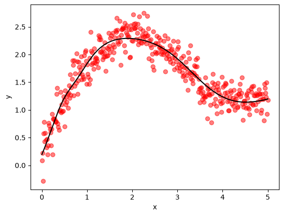
Here’s a visualization of the result.
plot_jax_output(θ, x_validate, y_validate)
24.6. Summary#
Here we compare the performance of the four different training approaches we explored in this lecture.
Summary of Training Methods:
                  Method  Runtime (s) Training MSE Validation MSE
                   Keras    21.582481     0.041501       0.046404
Pure JAX (hand-coded GD)     0.251214     0.039963       0.042119
         JAX + Optax SGD     0.249416     0.039963       0.042119
        JAX + Optax Adam     0.253332     0.035879       0.040869
All methods achieve similar validation MSE values (around 0.040-0.046).
At the time of writing, the MSEs from plain vanilla Optax and our own hand-coded SGD routine are identical.
The Adam optimizer achieves slightly better MSE by using adaptive learning rates.
Still, our hand-coded algorithm does very well compared to this high-quality optimizer.
Note also that the pure JAX implementations are significantly faster than Keras.
This is because JAX can JIT-compile the entire training loop.
Not surprisingly, Keras has more overhead from its abstraction layers.
24.7. Exercises#
Exercise 24.1
Try to reduce the MSE on the validation data without significantly increasing the computational load.
You should hold constant both the number of epochs and the total number of parameters in the network.
Currently, the network has 4 layers with output dimension \(k=10\), giving a total of \(251\) parameters.
You can experiment with:
Changing the network architecture
Trying different activation functions
Modifying the optimizer (e.g., learning rates, learning rate schedules, momentum, etc.)
Experimenting with different weight initialization strategies
Modifying the loss function (e.g., adding regularization)
Which combination gives you the lowest validation MSE?
Solution
Let’s implement and test several strategies.
Strategy 1: LR schedule and L2 regularization
Let’s keep the baseline network architecture and add a learning rate schedule with L2 regularization:
# Strategy 1: LR schedule and L2 regularization

def loss_fn_l2(
        θ: list,
        x: jnp.ndarray,
        y: jnp.ndarray,
        λ_l2: float
    ):
    " L2-regularized MSE loss. "
    mse = jnp.mean((f(θ, x) - y)**2)
    l2_penalty = 0.0
    for W, b in θ:
        l2_penalty += jnp.sum(W**2)
    return mse + λ_l2 * l2_penalty


loss_gradient_l2 = jax.grad(loss_fn_l2)


@partial(jax.jit, static_argnames=['config'])
def train_with_schedule_and_l2(
        θ: list,
        x: jax.Array,
        y: jax.Array,
        config: Config,
        λ_l2: float = 0.001
    ):
    """
    Train baseline network with learning rate schedule
    and L2 regularization.
    """
    epochs = config.epochs
    schedule = optax.exponential_decay(
        init_value=0.003,
        transition_steps=1000,
        decay_rate=0.5
    )

    solver = optax.adam(schedule)
    opt_state = solver.init(θ)

    def update(_, loop_state):
        θ_curr, opt_state_curr = loop_state
        grad = loss_gradient_l2(θ_curr, x, y, λ_l2)
        updates, opt_state_new = solver.update(
            grad, opt_state_curr, θ_curr
        )
        θ_new = optax.apply_updates(θ_curr, updates)
        return (θ_new, opt_state_new)

    initial_loop_state = θ, opt_state
    θ_final, _ = jax.lax.fori_loop(
        0, epochs, update, initial_loop_state
    )
    return θ_final

# Warmup
θ_l2 = initialize_network(param_key, config)
train_with_schedule_and_l2(θ_l2, x_train, y_train, config)

# Actual run
θ_l2 = initialize_network(param_key, config)
start_time = time()
θ_l2 = train_with_schedule_and_l2(θ_l2, x_train, y_train, config)
θ_l2[0].W.block_until_ready()
deep_l2_runtime = time() - start_time

deep_l2_mse = loss_fn(θ_l2, x_validate, y_validate)
print(f"Strategy 1 - LR schedule and L2 regularization")
print(f"  Runtime: {deep_l2_runtime:.2f}s")
print(f"  Validation MSE: {deep_l2_mse:.6f}")
print(f"  Improvement over Adam: {optax_adam_mse - deep_l2_mse:.6f}")
Strategy 1 - LR schedule and L2 regularization
  Runtime: 0.27s
  Validation MSE: 0.040850
  Improvement over Adam: 0.000019
Strategy 2: Baseline + Armijo line search
Let’s implement gradient descent with Armijo line search for adaptive step size selection:
# Strategy 2: Baseline architecture + Armijo line search
# Line search parameters
line_search_init_value = 0.01
line_search_backtrack_factor = 0.5
line_search_armijo_constant = 0.001
max_backtrack_steps = 20

@partial(jax.jit, static_argnames=['config'])
def train_jax_armijo_ls(
        θ: list,                    # Initial parameters (pytree)
        x: jnp.ndarray,             # Training input data
        y: jnp.ndarray,             # Training target data
        config: Config              # contains configuration data
    ):
    """
    Train model using gradient descent with Armijo line search.

    The Armijo line search adaptively finds a suitable step size at each
    iteration by ensuring sufficient decrease in the loss function.
    """
    epochs = config.epochs

    # Line search parameters
    α_init = line_search_init_value
    backtrack_factor = line_search_backtrack_factor
    armijo_c = line_search_armijo_constant

    def update_step(θ_current, x_data, y_data):
        current_loss = loss_fn(θ_current, x_data, y_data)
        g = loss_gradient(θ_current, x_data, y_data)

        # Squared Euclidean norm of gradient for Armijo condition
        g_norm_sq = jax.tree.reduce(
            lambda a, b: a + jnp.sum(b**2),
            g,
            initializer=0.0,
        )

        # Define the condition for the while_loop
        def cond_fn(loop_args):
            (α_val,
             current_loss_val,
             g_sq_sum,
             θ_orig,
             x_in,
             y_in,
             step_count) = loop_args

            loss_threshold = (
                current_loss_val - armijo_c * α_val * g_sq_sum
            )

            θ_candidate = jax.tree.map(
                lambda p, g_leaf: p - α_val * g_leaf,
                θ_orig,
                g,
            )
            loss_candidate = loss_fn(θ_candidate, x_in, y_in)
            return ((loss_candidate > loss_threshold)
                    & (step_count < max_backtrack_steps))

        # Define the body for the while_loop
        def body_fn(loop_args):
            (α_val,
             current_loss_val,
             g_sq_sum,
             θ_orig,
             x_in,
             y_in,
             step_count) = loop_args
            α_new = α_val * backtrack_factor
            step_count_new = step_count + 1
            return (α_new,
                    current_loss_val,
                    g_sq_sum,
                    θ_orig,
                    x_in,
                    y_in,
                    step_count_new)

        # Execute the Armijo line search using jax.lax.while_loop
        loop_state = jax.lax.while_loop(
            cond_fn,
            body_fn,
            (α_init, current_loss, g_norm_sq, θ_current, x_data, y_data, 0),
        )
        α_final = loop_state[0]

        # Update parameters with the chosen step size
        θ_new = jax.tree.map(
            lambda p, g_leaf: p - α_final * g_leaf,
            θ_current,
            g,
        )
        return θ_new

    # Main training loop (epochs)
    def outer_update(_, θ_curr):
        return update_step(θ_curr, x, y)

    θ_final = jax.lax.fori_loop(0, epochs, outer_update, θ)
    return θ_final

# Warmup
θ = initialize_network(param_key, config)
train_jax_armijo_ls(θ, x_train, y_train, config)

# Actual run
θ = initialize_network(param_key, config)
start_time = time()
θ_armijo = train_jax_armijo_ls(θ, x_train, y_train, config)
θ_armijo[0].W.block_until_ready()
armijo_runtime = time() - start_time

armijo_mse = loss_fn(θ_armijo, x_validate, y_validate)
print(f"Strategy 2 - Baseline + Armijo line search")
print(f"  Runtime: {armijo_runtime:.2f}s")
print(f"  Validation MSE: {armijo_mse:.6f}")
print(f"  Improvement over Adam: {optax_adam_mse - armijo_mse:.6f}")
Strategy 2 - Baseline + Armijo line search
  Runtime: 0.41s
  Validation MSE: 0.040810
  Improvement over Adam: 0.000058
Results Summary
Let’s compare all strategies:
Summary of Exercise Strategies:
                            Strategy  Runtime (s) Validation MSE  Improvement
              Baseline (Adam + tanh)     0.253332    0.040868692     0.000000
1. LR schedule and L2 regularization     0.269284     0.04085019     0.000019
    2. Baseline + Armijo line search     0.413090    0.040810395     0.000058
In terms of reducing loss on the validation data, the current winner is the Armijo line search strategy.
The Armijo backtracking line search is an adaptive step size method that dynamically adjusts the learning rate at each iteration to ensure sufficient decrease in the loss function.
Unlike fixed learning rates or predetermined schedules, it adapts to the local geometry of the loss landscape.
This strategy and its code were contributed by Matyas Farkas.