
10. Asset Pricing with nvmath-python#
GPU
This lecture was built using a machine with access to a GPU — although it will also run without one.
Google Colab has a free tier with GPUs that you can access as follows:
Click on the “play” icon top right
Select Colab
Set the runtime environment to include a GPU
10.1. Overview#
This lecture re-implements the asset pricing computations from An Asset Pricing Problem using nvmath-python, a Python library by NVIDIA that provides direct bindings to cuBLAS, cuSOLVER, cuFFT, and other CUDA math libraries.
The goal is twofold:
Show how to implement the same price-dividend ratio computation using nvmath, and verify that the output matches JAX.
Benchmark nvmath against JAX and NumPy/SciPy on the same problem.
For the economic theory and derivations, please refer to An Asset Pricing Problem. This lecture focuses purely on the computational implementation.
The core computation in both the simple and stochastic-volatility models reduces to solving a dense linear system
where \(K\) is a matrix built from model primitives. This maps naturally to:
nvmath.linalg.matmul— matrix-vector multiply (backed by cuBLASLt)nvmath.linalg.direct_solver— dense linear solve (backed by cuSOLVER)
Let’s check the GPU we are running:
!nvidia-smi
Sun Aug  2 19:36:18 2026
+-----------------------------------------------------------------------------------------+
| NVIDIA-SMI 580.105.08             Driver Version: 580.105.08     CUDA Version: 13.0     |
+-----------------------------------------+------------------------+----------------------+
| GPU  Name                 Persistence-M | Bus-Id          Disp.A | Volatile Uncorr. ECC |
| Fan  Temp   Perf          Pwr:Usage/Cap |           Memory-Usage | GPU-Util  Compute M. |
|                                         |                        |               MIG M. |
|=========================================+========================+======================|
|   0  Tesla T4                       On  |   00000000:00:1E.0 Off |                    0 |
| N/A   30C    P8             13W /   70W |       0MiB /  15360MiB |      0%      Default |
|                                         |                        |                  N/A |
+-----------------------------------------+------------------------+----------------------+

+-----------------------------------------------------------------------------------------+
| Processes:                                                                              |
|  GPU   GI   CI              PID   Type   Process name                        GPU Memory |
|        ID   ID                                                               Usage      |
|=========================================================================================|
|  No running processes found                                                             |
+-----------------------------------------------------------------------------------------+
In addition to JAX and Anaconda, this lecture needs:
!pip install quantecon
!pip install "nvmath-python[cu13]"
!pip install cupy-cuda13x
10.2. Imports#
import numpy as np
import cupy as cp
import scipy
import quantecon as qe
import matplotlib.pyplot as plt
import jax
import jax.numpy as jnp
import nvmath.linalg as nla
from collections import namedtuple
from time import perf_counter
We enable 64-bit floats in JAX to match NumPy and nvmath precision:
jax.config.update("jax_enable_x64", True)
10.3. The Simple Model#
10.3.1. Model setup#
We work with the simple asset pricing model from An Asset Pricing Problem. The state process \(\{X_t\}\) is a discretised AR(1) and the price-dividend ratio \(v\) satisfies
The unique solution is \(v = (I - K)^{-1} K\mathbf{1}\), provided the spectral radius of \(K\) is less than one.
Model = namedtuple('Model',
                   ('P', 'S', 'β', 'γ', 'μ_c', 'μ_d', 'σ_c', 'σ_d'))

def create_model(N=100,
                 ρ=0.9,
                 σ=0.01,
                 β=0.98,
                 γ=2.5,
                 μ_c=0.01,
                 μ_d=0.01,
                 σ_c=0.02,
                 σ_d=0.04):
    mc = qe.tauchen(N, ρ, σ)
    S = mc.state_values   # numpy array
    P = mc.P              # numpy array
    return Model(P=P, S=S, β=β, γ=γ, μ_c=μ_c, μ_d=μ_d, σ_c=σ_c, σ_d=σ_d)
10.3.2. JAX implementation#
The JAX implementation computes \(K\) on the GPU and uses
jax.scipy.linalg.solve to invert \((I - K)\).
def compute_K_jax(model):
    P, S, β, γ, μ_c, μ_d, σ_c, σ_d = model
    N = len(S)
    S_j = jnp.asarray(S)
    P_j = jnp.asarray(P)
    x = jnp.reshape(S_j, (N, 1))
    a = μ_d - γ * μ_c
    e = jnp.exp(a + (1 - γ) * x + (σ_d**2 + γ**2 * σ_c**2) / 2)
    return β * e * P_j

@jax.jit
def price_dividend_ratio_jax(model_arrays):
    P_j, S_j, β, γ, μ_c, μ_d, σ_c, σ_d = model_arrays
    N = len(S_j)
    sub = Model(P=P_j, S=S_j, β=β, γ=γ, μ_c=μ_c, μ_d=μ_d, σ_c=σ_c, σ_d=σ_d)
    K = compute_K_jax(sub)
    ones = jnp.ones(N)
    rhs = K @ ones
    v = jax.scipy.linalg.solve(jnp.eye(N) - K, rhs)
    return v
model = create_model()
# Push arrays to JAX device
jax_arrays = Model(
    P=jnp.asarray(model.P), S=jnp.asarray(model.S),
    β=model.β, γ=model.γ, μ_c=model.μ_c, μ_d=model.μ_d,
    σ_c=model.σ_c, σ_d=model.σ_d
)

# Warmup (triggers JIT compilation)
v_jax = price_dividend_ratio_jax(jax_arrays).block_until_ready()
print("JAX solution computed, shape:", v_jax.shape)
JAX solution computed, shape: (100,)
10.3.3. nvmath implementation#
The nvmath version builds \(K\) using CuPy (for elementwise GPU ops) and then delegates the matrix-vector multiply and linear solve to nvmath.
def compute_K_cupy(model):
    P, S, β, γ, μ_c, μ_d, σ_c, σ_d = model
    N = len(S)
    S_cp = cp.asarray(S)
    P_cp = cp.asarray(P)
    x = cp.reshape(S_cp, (N, 1))
    a = μ_d - γ * μ_c
    e = cp.exp(a + (1 - γ) * x + (σ_d**2 + γ**2 * σ_c**2) / 2)
    return β * e * P_cp

def price_dividend_ratio_nvmath(model):
    K = compute_K_cupy(model)
    N = K.shape[0]
    ones = cp.ones((N, 1), dtype=K.dtype)
    # nvmath.linalg.matmul: backed by cuBLASLt
    rhs = nla.matmul(K, ones).ravel()
    I_minus_K = cp.eye(N, dtype=K.dtype) - K
    # nvmath.linalg.direct_solver: backed by cuSOLVER (LU factorisation)
    v = nla.direct_solver(I_minus_K, rhs)
    cp.cuda.get_current_stream().synchronize()
    return v
v_nvmath = price_dividend_ratio_nvmath(model)
print("nvmath solution computed, shape:", v_nvmath.shape)
nvmath solution computed, shape: (100,)
10.3.4. Verification#
Let’s confirm both implementations produce the same price-dividend ratio:
v_jax_np = np.array(v_jax)
v_nvmath_np = cp.asnumpy(v_nvmath)

print(f"Max absolute difference: {np.max(np.abs(v_jax_np - v_nvmath_np)):.2e}")
print(f"Solutions match (allclose): {np.allclose(v_jax_np, v_nvmath_np, atol=1e-10)}")
Max absolute difference: 3.55e-15
Solutions match (allclose): True
10.3.5. Plot#
Here is the price-dividend ratio as a function of the state for several values of \(\gamma\):
fig, axes = plt.subplots(1, 2, figsize=(12, 4))

γs = np.linspace(2.0, 3.0, 5)
for ax, label, solver in zip(
        axes,
        ["JAX", "nvmath"],
        [
            lambda m: np.array(price_dividend_ratio_jax(
                Model(P=jnp.asarray(m.P), S=jnp.asarray(m.S),
                      β=m.β, γ=m.γ, μ_c=m.μ_c, μ_d=m.μ_d,
                      σ_c=m.σ_c, σ_d=m.σ_d))),
            lambda m: cp.asnumpy(price_dividend_ratio_nvmath(m)),
        ]):
    for γ in γs:
        m = create_model(γ=γ)
        v = solver(m)
        ax.plot(m.S, v, lw=2, alpha=0.6, label=rf"$\gamma = {γ:.1f}$")
    ax.set_title(label)
    ax.set_xlabel("state")
    ax.set_ylabel("price-dividend ratio")
    ax.legend(loc="upper right", fontsize=8)

fig.tight_layout()
plt.show()
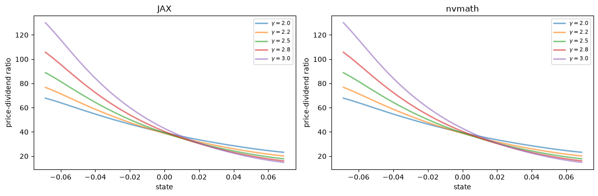
The plots are identical, confirming that both implementations agree.
10.4. The Stochastic Volatility Model#
The extended model adds time-varying volatility; see An Asset Pricing Problem for the derivation. The state is \(X_t = (H^c_t, H^d_t, Z_t)\) and the solution requires building a matrix \(A\) of size \((I \cdot J \cdot K) \times (I \cdot J \cdot K)\) and solving the same type of linear system.
SVModel = namedtuple('SVModel',
                     ('P', 'hc_grid',
                      'Q', 'hd_grid',
                      'R', 'z_grid',
                      'β', 'γ', 'bar_σ', 'μ_c', 'μ_d'))

def create_sv_model(β=0.98, γ=2.5,
                    I=14, ρ_c=0.9, σ_c=0.01,
                    J=14, ρ_d=0.9, σ_d=0.01,
                    K=14, bar_σ=0.01, ρ_z=0.9, σ_z=0.01,
                    μ_c=0.001, μ_d=0.005):
    mc = qe.tauchen(I, ρ_c, σ_c)
    hc_grid, P = mc.state_values, mc.P
    mc = qe.tauchen(J, ρ_d, σ_d)
    hd_grid, Q = mc.state_values, mc.P
    mc = qe.tauchen(K, ρ_z, σ_z)
    z_grid, R = mc.state_values, mc.P
    return SVModel(P=P, hc_grid=hc_grid,
                   Q=Q, hd_grid=hd_grid,
                   R=R, z_grid=z_grid,
                   β=β, γ=γ, bar_σ=bar_σ, μ_c=μ_c, μ_d=μ_d)
10.4.1. JAX implementation#
def compute_A_jax(sv_model, shapes):
    P, hc_grid, Q, hd_grid, R, z_grid, β, γ, bar_σ, μ_c, μ_d = sv_model
    I, J, K = shapes
    N = I * J * K
    hc = jnp.reshape(hc_grid, (I, 1, 1, 1, 1, 1))
    hd = jnp.reshape(hd_grid, (1, J, 1, 1, 1, 1))
    z  = jnp.reshape(z_grid,  (1, 1, K, 1, 1, 1))
    P_ = jnp.reshape(P,       (I, 1, 1, I, 1, 1))
    Q_ = jnp.reshape(Q,       (1, J, 1, 1, J, 1))
    R_ = jnp.reshape(R,       (1, 1, K, 1, 1, K))
    a = μ_d - γ * μ_c
    b = bar_σ**2 * (jnp.exp(2 * hd) + γ**2 * jnp.exp(2 * hc)) / 2
    κ = jnp.exp(a + (1 - γ) * z + b)
    return jnp.reshape(β * κ * P_ * Q_ * R_, (N, N))

def sv_pd_ratio_jax(sv_model_jax, shapes):
    P, hc_grid, Q, hd_grid, R, z_grid, β, γ, bar_σ, μ_c, μ_d = sv_model_jax
    I, J, K = shapes
    N = I * J * K
    A = compute_A_jax(sv_model_jax, shapes)
    ones = jnp.ones(N)
    v = jax.scipy.linalg.solve(jnp.eye(N) - A, A @ ones)
    return jnp.reshape(v, (I, J, K))

sv_pd_ratio_jax = jax.jit(sv_pd_ratio_jax, static_argnums=(1,))
sv_model = create_sv_model()
shapes = (sv_model.P.shape[0], sv_model.Q.shape[0], sv_model.R.shape[0])

# Put arrays on JAX device
sv_model_jax = SVModel(
    P=jnp.asarray(sv_model.P),       hc_grid=jnp.asarray(sv_model.hc_grid),
    Q=jnp.asarray(sv_model.Q),       hd_grid=jnp.asarray(sv_model.hd_grid),
    R=jnp.asarray(sv_model.R),       z_grid=jnp.asarray(sv_model.z_grid),
    β=sv_model.β, γ=sv_model.γ, bar_σ=sv_model.bar_σ,
    μ_c=sv_model.μ_c, μ_d=sv_model.μ_d
)

# Warmup
v_sv_jax = sv_pd_ratio_jax(sv_model_jax, shapes).block_until_ready()
print("JAX SV solution computed, shape:", v_sv_jax.shape)
JAX SV solution computed, shape: (14, 14, 14)
10.4.2. nvmath implementation#
def compute_A_cupy(sv_model, shapes):
    P, hc_grid, Q, hd_grid, R, z_grid, β, γ, bar_σ, μ_c, μ_d = sv_model
    I, J, K = shapes
    N = I * J * K
    hc = cp.reshape(cp.asarray(hc_grid), (I, 1, 1, 1, 1, 1))
    hd = cp.reshape(cp.asarray(hd_grid), (1, J, 1, 1, 1, 1))
    z  = cp.reshape(cp.asarray(z_grid),  (1, 1, K, 1, 1, 1))
    P_ = cp.reshape(cp.asarray(P),       (I, 1, 1, I, 1, 1))
    Q_ = cp.reshape(cp.asarray(Q),       (1, J, 1, 1, J, 1))
    R_ = cp.reshape(cp.asarray(R),       (1, 1, K, 1, 1, K))
    a = μ_d - γ * μ_c
    b = bar_σ**2 * (cp.exp(2 * hd) + γ**2 * cp.exp(2 * hc)) / 2
    κ = cp.exp(a + (1 - γ) * z + b)
    return cp.reshape(β * κ * P_ * Q_ * R_, (N, N))

def sv_pd_ratio_nvmath(sv_model, shapes):
    I, J, K = shapes
    N = I * J * K
    A = compute_A_cupy(sv_model, shapes)
    ones = cp.ones((N, 1), dtype=A.dtype)
    rhs = nla.matmul(A, ones).ravel()
    I_minus_A = cp.eye(N, dtype=A.dtype) - A
    v = nla.direct_solver(I_minus_A, rhs)
    cp.cuda.get_current_stream().synchronize()
    return cp.reshape(v, (I, J, K))
v_sv_nvmath = sv_pd_ratio_nvmath(sv_model, shapes)
print("nvmath SV solution computed, shape:", v_sv_nvmath.shape)
nvmath SV solution computed, shape: (14, 14, 14)
10.4.3. Verification#
v_sv_jax_np    = np.array(v_sv_jax)
v_sv_nvmath_np = cp.asnumpy(v_sv_nvmath)

print(f"Max absolute difference: {np.max(np.abs(v_sv_jax_np - v_sv_nvmath_np)):.2e}")
print(f"Solutions match (allclose): {np.allclose(v_sv_jax_np, v_sv_nvmath_np, atol=1e-10)}")
Max absolute difference: 1.14e-13
Solutions match (allclose): True
10.5. Benchmarks#
We now compare execution times across three backends:
Backend |
Library |
Device |
|---|---|---|
NumPy + SciPy |
|
CPU |
JAX |
|
GPU |
nvmath |
|
GPU |
10.5.1. Simple model: varying state-space size#
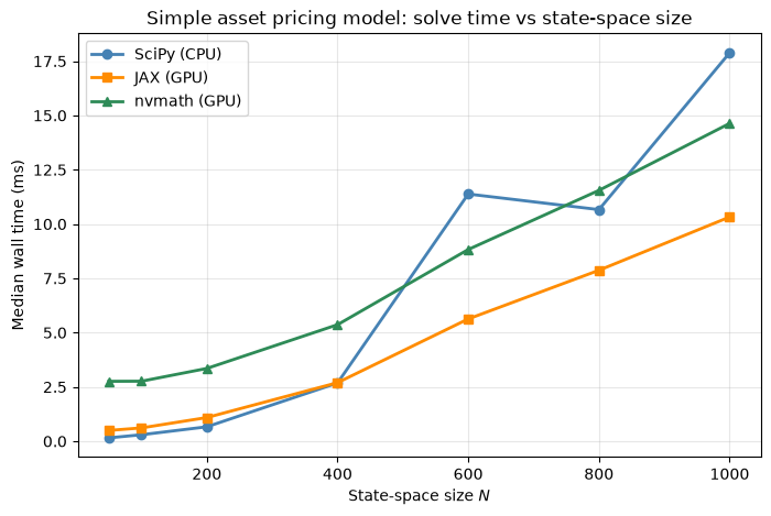
We benchmark the simple asset pricing model as the state-space size \(N\) grows.
def price_dividend_ratio_scipy(model):
    P, S, β, γ, μ_c, μ_d, σ_c, σ_d = model
    N = len(S)
    x = np.reshape(S, (N, 1))
    a = μ_d - γ * μ_c
    e = np.exp(a + (1 - γ) * x + (σ_d**2 + γ**2 * σ_c**2) / 2)
    K = β * e * P
    ones = np.ones(N)
    return scipy.linalg.solve(np.eye(N) - K, K @ ones)

def time_fn(fn, *args, n_runs=5):
    for _ in range(2):   # warmup
        fn(*args)
    times = []
    for _ in range(n_runs):
        t0 = perf_counter()
        fn(*args)
        times.append(perf_counter() - t0)
    return np.median(times)

N_values = [50, 100, 200, 400, 600, 800, 1000]
times_scipy  = []
times_jax    = []
times_nvmath = []

for N in N_values:
    m = create_model(N=N)

    # SciPy (CPU)
    t = time_fn(price_dividend_ratio_scipy, m)
    times_scipy.append(t)

    # JAX (GPU) — rebuild jax arrays each iteration
    m_jax = Model(P=jnp.asarray(m.P), S=jnp.asarray(m.S),
                  β=m.β, γ=m.γ, μ_c=m.μ_c, μ_d=m.μ_d,
                  σ_c=m.σ_c, σ_d=m.σ_d)
    t = time_fn(lambda x: price_dividend_ratio_jax(x).block_until_ready(), m_jax)
    times_jax.append(t)

    # nvmath (GPU)
    t = time_fn(price_dividend_ratio_nvmath, m)
    times_nvmath.append(t)

    print(f"N={N:4d}  scipy={times_scipy[-1]*1e3:7.2f}ms  "
          f"jax={times_jax[-1]*1e3:7.2f}ms  "
          f"nvmath={times_nvmath[-1]*1e3:7.2f}ms")
N=  50  scipy=   0.15ms  jax=   0.50ms  nvmath=   2.76ms
N= 100  scipy=   0.30ms  jax=   0.61ms  nvmath=   2.76ms
N= 200  scipy=   0.66ms  jax=   1.09ms  nvmath=   3.35ms
N= 400  scipy=   2.68ms  jax=   2.70ms  nvmath=   5.37ms
N= 600  scipy=  11.38ms  jax=   5.63ms  nvmath=   8.83ms
N= 800  scipy=  10.66ms  jax=   7.87ms  nvmath=  11.55ms
N=1000  scipy=  17.88ms  jax=  10.32ms  nvmath=  14.63ms
fig, ax = plt.subplots(figsize=(8, 5))

ax.plot(N_values, [t * 1e3 for t in times_scipy],
        'o-', lw=2, label='SciPy (CPU)', color='steelblue')
ax.plot(N_values, [t * 1e3 for t in times_jax],
        's-', lw=2, label='JAX (GPU)', color='darkorange')
ax.plot(N_values, [t * 1e3 for t in times_nvmath],
        '^-', lw=2, label='nvmath (GPU)', color='seagreen')

ax.set_xlabel("State-space size $N$")
ax.set_ylabel("Median wall time (ms)")
ax.set_title("Simple asset pricing model: solve time vs state-space size")
ax.legend()
ax.grid(True, alpha=0.3)
plt.show()
10.5.2. Stochastic volatility model: fixed grid, repeated timing#
Here we fix \(I = J = K = 14\) (state space of \(14^3 = 2744\)) and compare all three backends:
def sv_pd_ratio_scipy(sv_model, shapes):
    P, hc_grid, Q, hd_grid, R, z_grid, β, γ, bar_σ, μ_c, μ_d = sv_model
    I, J, K = shapes
    N = I * J * K
    hc = np.reshape(hc_grid, (I, 1, 1, 1, 1, 1))
    hd = np.reshape(hd_grid, (1, J, 1, 1, 1, 1))
    z  = np.reshape(z_grid,  (1, 1, K, 1, 1, 1))
    P_ = np.reshape(P,       (I, 1, 1, I, 1, 1))
    Q_ = np.reshape(Q,       (1, J, 1, 1, J, 1))
    R_ = np.reshape(R,       (1, 1, K, 1, 1, K))
    a = μ_d - γ * μ_c
    b = bar_σ**2 * (np.exp(2 * hd) + γ**2 * np.exp(2 * hc)) / 2
    κ = np.exp(a + (1 - γ) * z + b)
    A = np.reshape(β * κ * P_ * Q_ * R_, (N, N))
    ones = np.ones(N)
    return scipy.linalg.solve(np.eye(N) - A, A @ ones).reshape(I, J, K)

sv_model = create_sv_model()
shapes = (sv_model.P.shape[0], sv_model.Q.shape[0], sv_model.R.shape[0])
I, J, K = shapes
print(f"State-space size: {I}×{J}×{K} = {I*J*K}")

t_scipy  = time_fn(sv_pd_ratio_scipy, sv_model, shapes)
t_nvmath = time_fn(sv_pd_ratio_nvmath, sv_model, shapes)
t_jax    = time_fn(
    lambda: sv_pd_ratio_jax(sv_model_jax, shapes).block_until_ready()
)

print(f"\nSciPy  (CPU): {t_scipy  * 1e3:.1f} ms")
print(f"JAX    (GPU): {t_jax    * 1e3:.1f} ms")
print(f"nvmath (GPU): {t_nvmath * 1e3:.1f} ms")
print(f"\nSpeedup vs SciPy — JAX: {t_scipy/t_jax:.1f}×  nvmath: {t_scipy/t_nvmath:.1f}×")
State-space size: 14×14×14 = 2744

SciPy  (CPU): 280.1 ms
JAX    (GPU): 82.5 ms
nvmath (GPU): 86.2 ms

Speedup vs SciPy — JAX: 3.4×  nvmath: 3.2×
10.5.3. Scaling the stochastic volatility model#
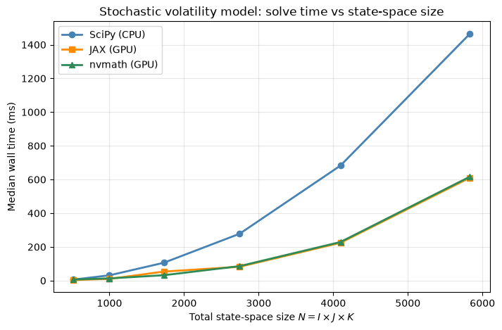
Let’s see how all three backends scale as the grid size increases:
grid_sizes = [8, 10, 12, 14, 16, 18]
sv_times_scipy  = []
sv_times_jax    = []
sv_times_nvmath = []

for g in grid_sizes:
    sv_m = create_sv_model(I=g, J=g, K=g)
    sh = (g, g, g)
    N_total = g**3

    sv_m_jax = SVModel(
        P=jnp.asarray(sv_m.P),       hc_grid=jnp.asarray(sv_m.hc_grid),
        Q=jnp.asarray(sv_m.Q),       hd_grid=jnp.asarray(sv_m.hd_grid),
        R=jnp.asarray(sv_m.R),       z_grid=jnp.asarray(sv_m.z_grid),
        β=sv_m.β, γ=sv_m.γ, bar_σ=sv_m.bar_σ,
        μ_c=sv_m.μ_c, μ_d=sv_m.μ_d
    )

    t = time_fn(sv_pd_ratio_scipy, sv_m, sh, n_runs=3)
    sv_times_scipy.append(t)

    t = time_fn(
        lambda: sv_pd_ratio_jax(sv_m_jax, sh).block_until_ready(),
        n_runs=3
    )
    sv_times_jax.append(t)

    t = time_fn(sv_pd_ratio_nvmath, sv_m, sh, n_runs=3)
    sv_times_nvmath.append(t)

    print(f"grid={g}  N={N_total:5d}  "
          f"scipy={sv_times_scipy[-1]*1e3:8.1f}ms  "
          f"jax={sv_times_jax[-1]*1e3:8.1f}ms  "
          f"nvmath={sv_times_nvmath[-1]*1e3:8.1f}ms")
grid=8  N=  512  scipy=     5.6ms  jax=     3.4ms  nvmath=     6.2ms
grid=10  N= 1000  scipy=    31.5ms  jax=    10.3ms  nvmath=    13.2ms
grid=12  N= 1728  scipy=   105.9ms  jax=    53.5ms  nvmath=    32.0ms
grid=14  N= 2744  scipy=   277.9ms  jax=    82.2ms  nvmath=    85.8ms
grid=16  N= 4096  scipy=   682.3ms  jax=   224.5ms  nvmath=   228.9ms
grid=18  N= 5832  scipy=  1464.8ms  jax=   610.8ms  nvmath=   616.6ms
N_totals = [g**3 for g in grid_sizes]

fig, ax = plt.subplots(figsize=(8, 5))
ax.plot(N_totals, [t * 1e3 for t in sv_times_scipy],
        'o-', lw=2, label='SciPy (CPU)', color='steelblue')
ax.plot(N_totals, [t * 1e3 for t in sv_times_jax],
        's-', lw=2, label='JAX (GPU)', color='darkorange')
ax.plot(N_totals, [t * 1e3 for t in sv_times_nvmath],
        '^-', lw=2, label='nvmath (GPU)', color='seagreen')

ax.set_xlabel("Total state-space size $N = I \\times J \\times K$")
ax.set_ylabel("Median wall time (ms)")
ax.set_title("Stochastic volatility model: solve time vs state-space size")
ax.legend()
ax.grid(True, alpha=0.3)
plt.show()
10.6. Summary#
In this lecture we ported the asset pricing computation from An Asset Pricing Problem to nvmath-python.
Key takeaways:
nvmath-python provides thin, direct bindings to NVIDIA’s CUDA math libraries (cuBLASLt for
matmul, cuSOLVER fordirect_solver).The same linear-algebra computation can be expressed almost identically in both JAX and nvmath; the matrix construction uses CuPy’s elementwise ops, while the solve step uses
nvmath.linalg.direct_solver.Both GPU backends produce results that agree with the CPU baseline to within floating-point precision.
The benchmark shows that both JAX and nvmath deliver significant speedups over NumPy + SciPy on a CPU, especially as the state space grows.
nvmath’s
DirectSolverclass (stateful API) can amortize the LU factorisation cost across multiple right-hand sides — useful when the same matrix is solved repeatedly with different \(v\) vectors.